4. Robot Localization
Part 1 (Sense)
This article explains one of the 2 main concepts discussed in Udacity's Self Driving Car -> Bayesian Thinking -> Lesson 11: Robot Localization.
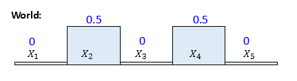
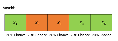
Situation: We have a 1 D world space with 5 different grid cells. They are colored red or green as shown below. Robot could be anywhere across this space, and all cells have equally likely chance. Thus we assume uniform probability distribution (1/5) = 0.2 for each cell. Also remember, the 1 D is cyclic, so if robot is in Cell 5, its next step is Cell 1. This is to keep our exercise simple.
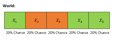
If Xi represents the cell location, then,
$$ \begin{align} p({{X}_{1}})=0.2\\ p({{X}_{2}})=0.2\\ p({{X}_{3}})=0.2\\ p({{X}_{4}})=0.2\\ p({{X}_{5}})=0.2 \end{align} $$
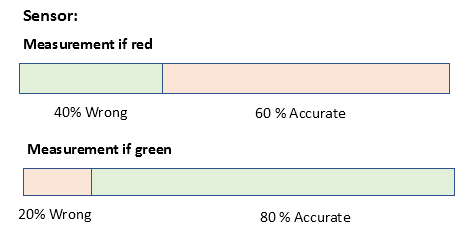
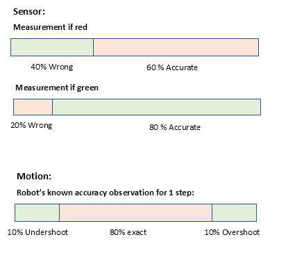
We also assume that, robot's sensor has accuracy as below.
Problem: Robot senses that the cell it is standing on, is "Red". What is the probability of robot location in each cell Xi?
Intuitively, then the probability of red cells should increase (as Robot mostly should be there), and green cells should decrease (as robot is not ideal and possibility of errors). Let us check mathematically. Using our earlier technique here, we could apply the evidence on prior situation as below.
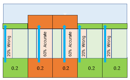
For 1st cell which is green, there is 20% chance that sensor read it as "red". Thus probability of location being green and sensor reading as "red" would be 20% out of 20% chance the green cell has. In other words, (0.2)(0.2) = 0.04. Similarly, we could calculate for all cells, and put in mathematical notation as below.
$\displaystyle \begin{array}{l}p({{X}_{1}}\cap Red)=\left( {0.2} \right)\left( {0.2} \right)=0.04\\p({{X}_{2}}\cap Red)=\left( {0.2} \right)(0.6)=0.12\\p({{X}_{3}}\cap Red)=\left( {0.2} \right)(0.6)=0.12\\p({{X}_{4}}\cap Red)=\left( {0.2} \right)\left( {0.2} \right)=0.04\\p({{X}_{5}}\cap Red)=\left( {0.2} \right)\left( {0.2} \right)=0.04\end{array}$
Summing up,
$$ \displaystyle \sum\limits_{{i=1}}^{n}{{p({{X}_{i}}\cap Red)}}=0.04+0.12+0.12+0.04+0.04=0.36 \tag{1} $$
We have thus calculated joint probability. Coming to posterior which is also the problem to be solved: Given the sensor reading is "red", what is the probability for each cell? We could readily use Bayes' theorem
$$ \displaystyle \begin{array}{l}p\left( {{{X}_{i}}|\text{Red}} \right)\text{ }=\frac{{p({{X}_{i}}\cap \text{Red})}}{{p(\text{Red})}}\\\\\text{ }=\frac{{p({{X}_{i}}\cap \text{Red})}}{{\sum\limits_{{k=1}}^{n}{{p({{X}_{k}}\cap \text{Red}}})}}\end{array} \tag{2} $$
Applying for each cell,
$ \displaystyle \begin{array}{l} p({{X}_{1}}|~\text{Red})=\left( {\frac{{0.04}}{{.36}}} \right)=0.111\\ p({{X}_{2}}|~\text{Red})=\left( {\frac{{0.12}}{{.36}}} \right)=0.333\\ p({{X}_{3}}|~\text{Red})=\left( {\frac{{0.12}}{{.36}}} \right)=0.333\\ p({{X}_{4}}|~\text{Red})=\left( {\frac{{0.04}}{{.36}}} \right)=0.111\\ p({{X}_{5}}|~\text{Red})=\left( {\frac{{0.04}}{{.36}}} \right)=0.111 \end{array}$
Note that, posterior probability adds up to 1 again like prior.
$ \displaystyle \sum\limits_{{i=1}}^{n}{{p\left( {{{X}_{i}}|\text{Red}} \right)}}=1$
Also, again using Baye's theorem for RHS for (2), we could re write it as below.
$$ \displaystyle \begin{array}{l}p\left( {{{X}_{i}}|\text{Red}} \right)=\frac{{p({{X}_{i}}\cap \text{Red})}}{{\sum\limits_{{k=1}}^{n}{{p({{X}_{k}}\cap \text{Red)}}}}}\\\\\text{ }=\frac{{p(\text{Red }\!\!|\!\!\text{ }{{X}_{i}})p({{X}_{i}})}}{{\sum\limits_{{k=1}}^{n}{{p(\text{Red }\!\!|\!\!\text{ }{{X}_{k}})p({{X}_{k}})}}}}\end{array} $$
Thus finally our posterior probability distribution in our visual summary:

Note, that as intuitively imagined earlier, the probability for red cells have increased from 0.2 to 0.33 while the green cells has their probability decreased from 0.2 to 0.111. Now robot is more certain of its location :)
So remember, each time, robot senses' its certainty increases. Its more sure of its location.
Food for thought: What happens to the probability distribution if we ask robot to keep sensing for many times. Intuitively, then the red cells each should achieve 0.5 probability eventually and rest going to 0. Let us check this out pro grammatically after implementing sense function.
Python Implementation:
Suppose,
p = list of prior probabilities of all cells world = list of color of each cell in same order (kinda map given to robot) Z = robot's measurement (in our test case, 'red') pHit = probability of robot correctly sensing red when its actually red pMiss = probability of robot wrongly sensing red, when its actually green
then,
- for each element in p, we could simply calculate the joint probability first by multiplying with pHit, if cell is red, or pMiss if cell is green
- calculate the p(Red) by summing up the joint probabilities
- calculate prior probability by diving each element again with the sum
Thus the implementation is as follows (slightly different than Udacity's as we derived directly from logic without referring it).
p=[0.2, 0.2, 0.2, 0.2, 0.2]
world=['green', 'red', 'red', 'green', 'green']
pHit = 0.6
pMiss = 0.2
def sense(p, Z):
    """
    p = initial probability distribution list
    Z = each measurement
    q = new normalized distribution list
    """
    q = []
    for each_index in range(len(p)):
        if (world[each_index] == Z):
            q.append(p[each_index]<em>pHit)
        else:
            q.append(p[each_index]</em>pMiss)
    total = sum(q)
    q = [ x/total for x in q]
    return q

print("Prior probability: " + str(p))
print("Posterior probability: " + str(sense(p,'red')))
Output:

Coming back to food for thought, we could simulate asking robot to sense so many times by calling sense repeatedly with measurement as 'red'. Result is as expected.
p=[0.2, 0.2, 0.2, 0.2, 0.2]
print("Prior probability: " + str(p))
for i in range(1000):
    p = sense(p, 'red')
print("Posterior probability: " + str(sense(p,'red')))
Output:
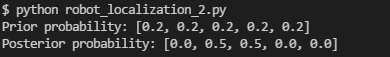
So when you keep sensing new information, your certainty increases.
Part 2 (Move)
We will now see, what happens to probability distributions when robot moves.
Situation: We have a 1 D world space with 5 grid cells. Robot could be anywhere across this space and we assume a probability distribution like below (say, due to a previous sense function, few cells have more probability). That is, we assume robot has equally likely chance of being either at X2 or X4, and not anywhere else. Also world is cyclic that is after X5 , next cell is X1.
If Xi represents the cell location, then
$$ \displaystyle \begin{array}{l}p({{X}_{1}})=0\\p({{X}_{2}})=0.5\\p({{X}_{3}})=0\\p({{X}_{4}})=0.5\\p({{X}_{5}})=0\end{array} \tag{1} $$
Let us also assume robot moves in 2 steps, always to its right side, and it's motion accuracy as below.

Problem: Robot moves 2 steps right. What is the probability of robot location in each cell Xi ? Appears like posterior, but we will get to that soon.
Intuitively, since the robot as per our assumption could have moved only from X2 or X4 , their probability should decrease, and probable target cells' probability increase. Generically, any cell's probability, depends on robot arriving at it from adjacent cells' either by undershoot or exact or overshoot from cells' left side (caz robot always move in right direction). For eg, For X1 ,the only way robot would have arrived is if robot was earlier in X4 and did exact 2 steps motion to its right.
Since both probability (prior and posterior) is on same sample space "location" we shall differentiate the event by time notation for easier understanding. Further, there is also mix up of probabilities (one cell might receive robot from more than one source. For eg, X5 might have received either by robot undershooting from X4 or overshooting from X2 .
We will thus divide the cases by all possible current locations, calculate the probabilities individually and then add up. Don't worry, it is for this purpose, we assumed only 2 locations having prior probability of having the robot. We have thus only 2 cases as below.
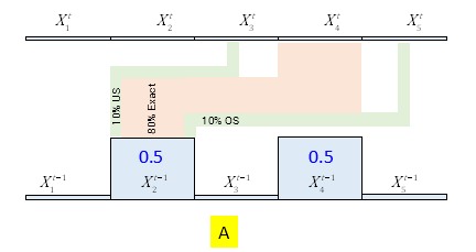
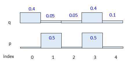
Case A: Robot moving from X2 . Including time notation, we could visualize its further movement with probabilities as below.
For example, out of 50% of being at X2, robot has 10% chance of ending up at X3 after its movement, as it might undershoot. Other locations could be understood in similar manner.
Case B: Robot moving from X4. Its visualization could be as follows.

Now, for each cell's probability, we could calculate simply $ \displaystyle p(A\cup B)$ as below.
$$ \displaystyle p(A\cup B)=p(A)+p(B)-p(A\cap B)=p(A)+p(B) \tag{2} $$
$ \displaystyle p(A\cap B)=0$ because, robot could have moved either from X2 or X4 not both. (We are not including quantum effects here ;).
Now we can derive individual cell's probabilities in both cases as below. For eg, in case A, $ \displaystyle p(X_{1}^{t})=0$ because, there is no way, robot could have arrived at X1 from X2 . Similarly for others. Make sure you fully able to comprehend below equations , as we would generalize this shortly.
$ \displaystyle p(A)$:
$$ \displaystyle \begin{array}{l}p(X_{1}^{t})=0\\p(X_{2}^{t})=0\\p(X_{3}^{t})=p(X_{2}^{{t-1}})p(X_{3}^{t}|X_{2}^{{t-1}})=p(X_{2}^{{t-1}})(0.1)=(0.5)(0.1)=0.05\\p(X_{4}^{t})=p(X_{2}^{{t-1}})p(X_{4}^{t}|X_{2}^{{t-1}})=p(X_{2}^{{t-1}})(0.8)=(0.5)(0.8)=0.40\\p(X_{5}^{t})=p(X_{2}^{{t-1}})p(X_{5}^{t}|X_{2}^{{t-1}})=p(X_{2}^{{t-1}})(0.1)=(0.5)(0.1)=0.05\end{array} \tag{3} $$
$ \displaystyle p(B)$:
$$ \displaystyle \begin{array}{l}p(X_{1}^{t})=p(X_{4}^{{t-1}})p(X_{1}^{t}|X_{4}^{{t-1}})=p(X_{4}^{{t-1}})(0.8)=(0.5)(0.8)=0.40\\p(X_{2}^{t})=p(X_{4}^{{t-1}})p(X_{2}^{t}|X_{4}^{{t-1}})=p(X_{4}^{{t-1}})(0.1)=(0.5)(0.1)=0.05\\p(X_{3}^{t})=0\\p(X_{4}^{t})=0\\p(X_{5}^{t})=p(X_{4}^{{t-1}})p(X_{5}^{t}|X_{4}^{{t-1}})=p(X_{4}^{{t-1}})(0.1)=(0.5)(0.1)=0.05\end{array} \tag{4} $$
Combining (3)and (4) using (2), we thus could arrive at final probabilities of each cell.
$$ \displaystyle \begin{array}{l}p(X_{1}^{t})=p(X_{4}^{{t-1}})p(X_{1}^{t}|X_{4}^{{t-1}})=p(X_{4}^{{t-1}})(0.8)=(0.5)(0.8)=0.40\\p(X_{2}^{t})=p(X_{4}^{{t-1}})p(X_{2}^{t}|X_{4}^{{t-1}})=p(X_{4}^{{t-1}})(0.1)=(0.5)(0.1)=0.05\\p(X_{3}^{t})=p(X_{2}^{{t-1}})p(X_{3}^{t}|X_{2}^{{t-1}})=p(X_{2}^{{t-1}})(0.1)=(0.5)(0.1)=0.05\\p(X_{4}^{t})=p(X_{2}^{{t-1}})p(X_{4}^{t}|X_{2}^{{t-1}})=p(X_{2}^{{t-1}})(0.8)=(0.5)(0.8)=0.40\\\\p(X_{5}^{t})=p(X_{2}^{{t-1}})p(X_{5}^{t}|X_{2}^{{t-1}})+p(X_{4}^{{t-1}})p(X_{5}^{t}|X_{4}^{{t-1}})\\=p(X_{2}^{{t-1}})(0.1)+p(X_{4}^{{t-1}})(0.1)=(0.5)(0.1)+(0.5)(0.1)=0.1\end{array} \tag{5}$$
Voila. We derived final probabilities. Visualizing,
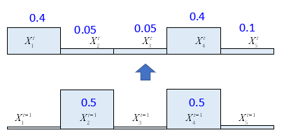
Note that, all $ \displaystyle {p(X_{i}^{t})}$ add up to 1. That is,
$$ \displaystyle \sum\limits_{{k=1}}^{n}{{p(X_{i}^{t})=1}}$$
Thus, $ \displaystyle {p(X_{i}^{t})}$ is already a posterior probability or same as joint probability as no distinguishing between them needed. This is an important inference. Further, "movement" only caused the distribution to "shift" in direction of robot to other cells, unlike our earlier case "sense".
Food for thought: Try a simpler case as below for move example, with 100% certainty for initial location and exact movement of robot with no under or overshoot and these would be much more evident.

Generalization:
Coming back to our initial example, lets examine say X1 . We know, robot could have come to it only from X4 in our case, so possibility from all other cells would be 0.
$ \displaystyle p(X_{1}^{t})=0+p(X_{4}^{{t-1}})p(X_{1}^{t}|X_{4}^{{t-1}})$
If we try to generalize case of X1 to include all locations, it would be like below and only that except $ \displaystyle p(X_{4}^{{t-1}})p(X_{1}^{t}|X_{4}^{{t-1}})$, other factors ended up 0 as below. For eg, $ \displaystyle p(X_{1}^{t}|X_{2}^{{t-1}})$ is 0 because, no way robot would have come from X2 to X1.
$$ \displaystyle \begin{array}{l}p(X_{1}^{t})=p(X_{1}^{{t-1}})p(X_{1}^{t}|X_{1}^{{t-1}})+p(X_{2}^{{t-1}})p(X_{1}^{t}|X_{2}^{{t-1}})\\+p(X_{3}^{{t-1}})p(X_{1}^{t}|X_{3}^{{t-1}})+p(X_{4}^{{t-1}})p(X_{1}^{t}|X_{4}^{{t-1}})+p(X_{5}^{{t-1}})p(X_{1}^{t}|X_{5}^{{t-1}})\\\\=p(X_{1}^{{t-1}})(0)+p(X_{2}^{{t-1}})(0)+p(X_{3}^{{t-1}})(0)+p(X_{4}^{{t-1}})(0.1)+p(X_{5}^{{t-1}})(0)\\=p(X_{1}^{{t-1}})(0)+p(X_{2}^{{t-1}})(0)+p(X_{3}^{{t-1}})(0)+(0.5)(0.8)+p(X_{5}^{{t-1}})(0)=0.40\end{array} \tag{6} $$
Generalizing this further for any cell Xi, we get,
$$ \displaystyle \begin{array}{l}p(X_{i}^{t})=p(X_{1}^{{t-1}})p(X_{i}^{t}|X_{1}^{{t-1}})+p(X_{2}^{{t-1}})p(X_{i}^{t}|X_{2}^{{t-1}})\\+p(X_{3}^{{t-1}})p(X_{i}^{t}|X_{3}^{{t-1}})+p(X_{4}^{{t-1}})p(X_{i}^{t}|X_{4}^{{t-1}})+p(X_{5}^{{t-1}})p(X_{i}^{t}|X_{5}^{{t-1}})\end{array} \tag{7} $$
Formulating, we get:
$$ \displaystyle p(X_{i}^{t})=\sum\limits_{{k=1}}^{n}{{p(X_{k}^{{t-1}})p(X_{i}^{t}|X_{k}^{{t-1}})}} \tag{8} $$
This equation above is called "Theorem of Total Probability". The above equation is responsible for shifting of the distribution and this mechanism is generally called "convolution". Sounds cool, eh?!
Python Implementation:
Assume,
p = list of prior probabilities of all cells
U = robot's movement in steps (in our case, its 2)
pExact = probability of robot exactly finishes 2 steps and ends up at Uth (2nd in our case) cell to its right
pUndershoot = probability of robot undershoots, and ends up at (U-1)th cell (1st cell in our case) to its right
pOvershoot = probability of robot overshoots and ends up at (U+1)th cell (3rd cell in our case) to its right
The approach is little bit tricky. So let's hard code for our logic and see if we could derive general code out of it. Let us take another list 'q' same size as p and try to calculate case A. We could visualize as below.

Then we could readily calculate, non zero values of q from diagram as below.
q[2] = p[1](0.1) = (0.5)(0.1) = 0.05 q[3] = p[1](0.8) = (0.5)(0.8) = 0.40 q[4] = p[1](0.1) = (0.5)(0.1) = 0.05(9)
Now the 'new' q would be as below.

Now case B, but on 'new' q, because we should not lose old q values as probabilities add up. Recall (2).
q[0] = p[3](0.8) + q[0] = (0.5)(0.8) + 0 = 0.40 q[1] = p[3](0.1) + q[1] = (0.5)(0.1) + 0 = 0.05 q[4] = p[3](0.1) + q[4] = (0.5)(0.1) + 0.05 = 0.10(10)
Note how case A and B added up for q[4]. The resultant distribution might look like this:
Generalizing from both above equations, and re writing again we get:
q[2] = p1 + q[2] = (0.5)(0.1) + 0 = 0.05 #undershoot
q[3] = p1 + q[3] = (0.5)(0.8) + 0 = 0.40 #exact
q[4] = p1 + q[4] = (0.5)(0.1) + 0 = 0.05 #overshoot
q[4] = p3 + q[4] = (0.5)(0.1) + 0.05 = 0.10 #undershoot
q[0] = p3 + q[0] = (0.5)(0.8) + 0 = 0.40 #exact
q[1] = p3 + q[1] = (0.5)(0.1) + 0 = 0.05 #overshoot
Note that, we calculated only for 2 cases involving p[1] and p[3], as it was evident from our case. We could extend this for all p elements. Visualize to imagine target q elements for each element of p to calculate its probabilities.
q[1] = p0 + q[1]
q[2] = p0 + q[2]
q[3] = p0 + q[3]
q[2] = p1 + q[2]
q[3] = p1 + q[3]
q[4] = p1 + q[4]
q[3] = p2 + q[3]
q[4] = p2 + q[4]
q[0] = p2 + q[0]
q[4] = p3 + q[4]
q[0] = p3 + q[0]
q[1] = p3 + q[1]
q[0] = p4 + q[0]
q[1] = p4 + q[1]
q[2] = p4 + q[2]
Some might have already observed an emerging pattern. Let us quickly check the code, if this works fine before we generalize.
In below code, we just create an empty q list of same size as p, (and a temp list for undershoot/exact/overshoot probabilities). Then we update for each element p with above logic and then simply return the updated q.
p=[0, 0.5, 0, 0.5, 0]
pExact = 0.8
pOvershoot = 0.1
pUndershoot = 0.1
def move(p, U):
"""
p = given probability distribution list
U = amount of steps robot has moved to right (assumed as right for now)
"""
# INEXACT MOTION
q = [ 0 for _ in p ]
temp = [pUndershoot, pExact, pOvershoot]
q[1] = p[0]<em>temp[0] + q[1]
q[2] = p[0]</em>temp[1] + q[2]
q[3] = p[0]*temp[2] + q[3]
<pre><code>q[2] = p[1]*temp[0] + q[2]
q[3] = p[1]*temp[1] + q[3]
q[4] = p[1]*temp[2] + q[4]
q[3] = p[2]*temp[0] + q[3]
q[4] = p[2]*temp[1] + q[4]
q[0] = p[2]*temp[2] + q[0]
q[4] = p[3]*temp[0] + q[4]
q[0] = p[3]*temp[1] + q[0]
q[1] = p[3]*temp[2] + q[1]
q[0] = p[4]*temp[0] + q[0]
q[1] = p[4]*temp[1] + q[1]
q[2] = p[4]*temp[2] + q[2]
return q
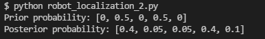
print("Prior probability: " + str(p))
print("Posterior probability: " + str(move(p,2)))
Output:
Great, this works. Now let us condense it to generalize. We need to run for all elements of p, so that calls for a for loop. Tricky part is the indexing of q. Check the flow of q indexes. Its { (1,2,3) , (2,3,4), (3,4,0) ...}
If we run a for loop, the p's index could be used to calculate q's index by using undershoot, exact and overshoot target cell location relative to current p's index.
For example, in case of p[1], we could also re write as below (remember, U = 2 in our case).
q[ (1 + (U-1)) ] = p[1]temp[0] + q[ (1 + (U-1)) ]
q[ (1 + U) ] = p[1]temp[1] + q[ (1 + U) ]
q[ (1 + (U+1)) ] = p[1]*temp[2] + q[ (1 + (U+1)) ]
You can verify that, substituting for U, you get the same as what you got earlier. That is,
q[2] = p[1]temp[0] + q[2]
q[3] = p[1]temp[1] + q[3]
q[4] = p[1]*temp[2] + q[4]
Good. But what about edge elements. Try doing the same for p[3] with U=2.
q[ (3 + (U-1)) ] = p[3]temp[0] + q[ (3 + (U-1)) ]
q[ (3 + U) ] = p[3]temp[1] + q[ (3 + U) ]
q[ (3 + (U+1)) ] = p[3]*temp[2] + q[ (3 + (U+1)) ]
becomes
q[ 4 ] = p[3]temp[0] + q[ 4 ]
q[ 5 ] = p[3]temp[1] + q[ 5 ]
q[ 6 ] = p[3]*temp[2] + q[ 6 ]
Oh ho. You can see, this calculation simply overflows beyond max index of q. We said, our 1D is cyclic. Thus we should be getting,
q[4] = p[3]temp[0] + q[4]
q[0] = p[3]temp[1] + q[0]
q[1] = p[3]*temp[2] + q[1]
So after q[4], we should get q[0]. Modulo operator comes to the rescue here.
Note that, 5 % 5 = 0, 6 % 5 = 1, the exact numbers we need. Mod does not affect when numerator is smaller. for eg, 4 % 5 is still 4. Perfect! Substituting that, and taking off the index calculations for q for brevity, we get the logic as below.
undershoot_index = (i + (U-1)) % len(p)
exact_index = (i + (U)) % len(p)
overshoot_index = (i + (U+1)) % len(p)
q[ undershoot_index ] = p[i]temp[0] + q[ undershoot_index ]
q[ exact_index ] = p[i]temp[1] + q[ exact_index ]
q[ overshoot_index ] = p[i]*temp[2] + q[ overshoot_index ]
Let us now try this generalized approach. This time, we use a for loop, and inside that, above logic.
 p=[0, 0.5, 0, 0.5, 0]
 pExact = 0.8
 pOvershoot = 0.1
 pUndershoot = 0.1
 def move(p, U):
 """
 p = given probability distribution list
 U = amount of steps robot has moved to right (assumed as right for now)
 """
 ### INEXACT MOTION
 q = [ 0 for _ in p ]
 temp = [pUndershoot, pExact, pOvershoot]

for i in range(len(p)):
 undershoot_index = (i + (U-1)) % len(p)
 exact_index = (i + (U)) % len(p)
 overshoot_index = (i + (U+1)) % len(p)
 q[ undershoot_index ] = p[i]<em>temp[0] + q[ undershoot_index ]
 q[ exact_index ] = p[i]</em>temp[1] + q[ exact_index ]
 q[ overshoot_index ] = p[i]*temp[2] + q[ overshoot_index ]

return q

print("Prior probability: " + str(p))
 print("Posterior probability: " + str(move(p,2)))
Output:
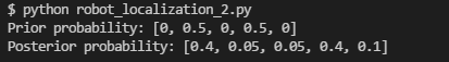
It works :)
You could try with different values of p, U and see that the program works.
Interesting observation: What if the robot keeps on moving 2 steps at a time. Intuitively over time, the uncertainty approaches maximum: robot is equally likely to be present in any cell. In other words, each cell would have (1/5) = 0.2 probability in our case of 1 D space of 5 cells.
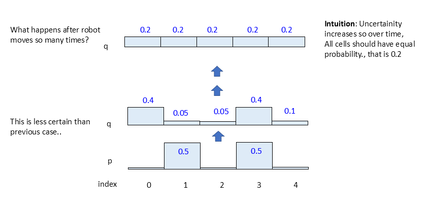
Let us check the code, calling the move for, say 1000 times.
p=[0, 0.5, 0, 0.5, 0]
print("Prior probability: " + str(p))
for i in range(1000):
    p = move(p,2)
print("Posterior probability: " + str(move(p,2)))
Output:

We got 0.2 for all cells :)
So when you just move every time, without 'sensing' any new information, uncertainty increases.
Part 3 (Combination)
We have implemented two important functions for robot localization. Sense gains new information and increases certainty of robot's localization. Move loses information increasing uncertainty of robot's localization. So both should be alternatively and accordingly used for successful navigation of robots.
Note when we say sense or move, we only update probability distribution given robot's capability for sense and motion. We did not operate robot directly yet.That said, let us again re imagine our 1 D world again. Note also, we assume U = 1, that is, robot moving 1 cell at a time.
Suppose,
- Robot senses 'red'
- Move one step to right
- Robot senses 'green'
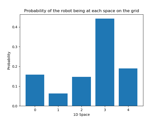
What would be its current location intuitively? By looking at the map, we could say, its X4. But how could robot with all its sense and move inaccuracies fare in detecting that location? Let us calculate the resultant probability distribution.
#Just for visualization
import matplotlib.pyplot as plt
def output_map(grid):
"""
outputs a bar chart showing the probabilities of each grid space
"""
x_labels = []
for index in range(len(grid)):
x_labels.append(index)
plt.bar(x_labels, grid)

<h1>Create names on the axes</h1>

plt.title('Probability of the robot being at each space on the grid')
plt.xlabel('1D Space')
plt.ylabel('Probability')
plt.show(block=True)

#initial probability
p=[0.2, 0.2, 0.2, 0.2, 0.2]

#sense
world=['green', 'red', 'red', 'green', 'green']
pHit = 0.6
pMiss = 0.2

#move
pExact = 0.8
pOvershoot = 0.1
pUndershoot = 0.1

#our operation
print("Prior probability: " + str(p))
p = sense(p, 'red')
p = move(p , 1)
p = sense(p , 'green')
print("Posterior probability: " + str(p))
output_map(p)
Output:

I have also included a visualization, so the result is obvious.